Test of Liouville

Note

This is a log book of the apps121025_test_liouville appliation set. Later summarize and move to proper directory in sphinx documentation.

Note

Note for developer. If no figures are made, you hae to run the script in apps121025_test_liouville.

Introduction

Due to textbooks, it is said that phase space volume is conserved along the trajectory. Yes, I have learned as such, but I have not yet “validated”. This document provides validation of the volume of the element in phase space along trajectory.

Method

I used trajectory tracing of Kepler motion. Kepler trajectory is calculated as a fourth order Runge-Kutta solver in 6-D dimension. I used scipy.integral.odeint for integration.

For simplicity, 4-D dimension problems are solved. This means that the position of each particles have (x, y) component and the velocity has (vx, vy) component.

The implementations are in apps121025_test_liouville.

Kepler motion

A single particle trajectory in x-y and vx-vy plane is shown here.

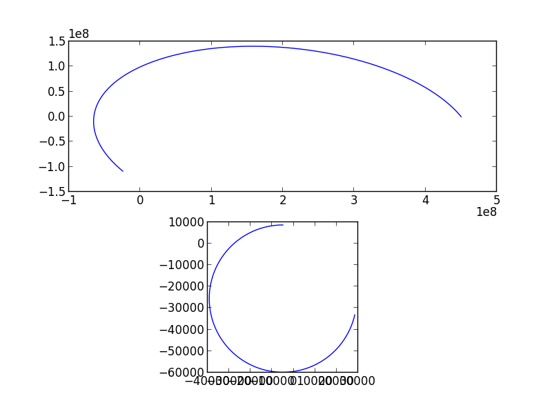
Top panel is the real space, starting from (4.5e8, 0) with velocity of 10 km/s (120 deg off). The calculation was done for 3e4 sec.

Here it is noted that the integral was done in MKSA unit. Some concerns on numerical error occurred to me. Namely, it is a large number difference in the real space (1e8 order) and the velocity space (1e4 order).

Now, I simply normalized the equation of motion. This works very well, so that all the parameters is about 1, and the multiple of gravity constant and center mass went to 1.

\[\frac{dv}{dt} = -GM \frac{r}{|r|^3}\]

\[\frac{dr}{dt} = v\]

The normalizations below are applied.

\[\hat{r} = \sqrt{GM}r\]

\[\hat{v} = \sqrt[4]{GM}v\]

\[\hat{t} = \sqrt[4]{GM}t\]

Now we get a normalized equation of motion.

\[\frac{d\hat{v}}{d\hat{t}} = - \frac{\hat{r}}{|\hat{r}|^3}\]

\[\frac{d\hat{r}}{d\hat{t}} = \hat{v}\]

(From now on I remove the hat notation for simplicity.)

Now the corresponding trajectories of a single particle become:

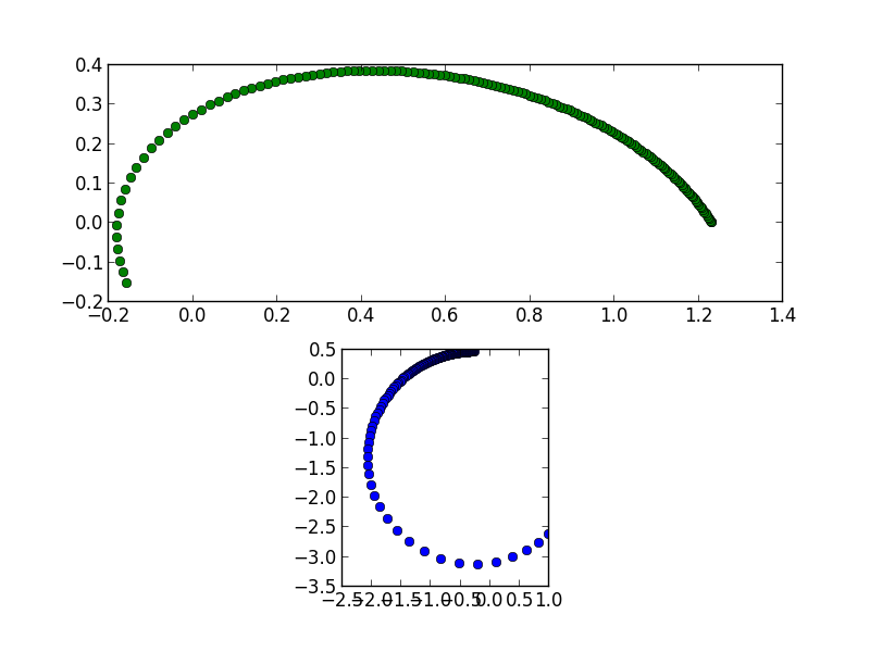
The result gives approximately same solutions to the one before, but both the numbers of position and velocity are the order of 1.

Test particle simulation

Now, to be validated is the conservation of \(dxdydv_xdv_y\) in the normalized phase space. So I used test particle runs to validate the conservation.

Reference particle

Reference particle is the particle that has a certain initial position (r0) and velocity (v0). I used the particle shown above. The initial position and velocity is both very close to 1.

Setup at t=0

I made 500 test particles with a random distribution uniformly in both position (r0 + dr) and velocity (v0 + dv). Here, dr and dv is taken 0.001 thus the “resolution” is ~0.1 %.

Result at t~1

After a certain time (t~1), particle trajectories are traced and obtain the position (r1) and the velocity (v1). They are plotted in the following.

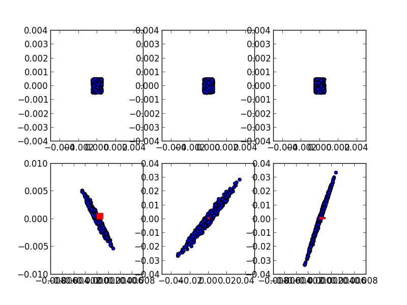
Top three panels are for t=0, and the bottom three panels are for t=1. From left to right, “x-y”, “vx-vy”, “x-vy” of 500 particles are drawn. Red boxes in the bottom correspond to the initial occupation of the particles (identical to the volume above).

Looking at these figures, the volume occupation at t=1 (blue regions in bottom panels) is much much much bigger than the volume at t=0 (red regions in bottom panels). Intuitively, this result is NOT CONSISTENT with the phase space volume conservation because the result looks to suggest \(dxdydv_xdv_y(t=0) << dxdydv_xdv_y(t=1)\).

What’s wrong?

Something wrong… myself or Liouville?

One possible idea is the numerical error. I tried different parameter, such as dx or dvx or integration time and so on. The possiblity is not very high.

Another possibility? How about assuming just an appearent effect. Obviously the phase space “volume” is defined in 4-D space (or in general 6-D space). I can only plot 2-D. The “volume” in above plot does not LOOK conserved, but this could be only the projection problem. If I can calculate the exact volume, probably it is conserved.

Now, I must check the “volume” in 4-D space without any projection.

General volume

Ok, now we consider the evolution of “volume” along the orbit. But, what is volume? Good question. The problem is that we should handle 4-D space.

Let me consider lower demension first. For 2-D space, 2 vectors from the origin will make the area of parallelogram (or triangle). For 3-D space, 3 vectors from the origin will make the volume of hexahedron.

Ok for now, “For 4-D space, 4 vectors from the origin will make the (super-)volume of (super)hexahedron.” Not bad. Well, but how?

Graminan

A search in the internet provided a hint: It is Gram’s matrix. http://staff.miyakyo-u.ac.jp/~h-uri/blog/archive/lecture/biseki/2003/haifu/volume.pdf (Sorry this is japanese document.)

Summarizing the above pdf:

• Consider n-dimensional vector space.

• Take m vectors in the space, \(\vec{a_1}, \vec{a_2}, ..., \vec{a_m}\). 0 <= m <= n.

• The m*x*m size matrix, \(G_m = G_m[i,j] = \vec{a_i}\cdot\vec{a_j}\), is called Gram’s matrix

• The Gram’s matrix, Gij, is symmetrix matrix. (More specifically, it is positive definite symmetrix matrix.)

• The determinant of the Gram’s matrix is called “Graminan”.

• The area of the parallelogram defined by \(\vec{a_1}, \vec{a_2}\) is \(\sqrt{det G_2}\).

• The volume of the hexahedron defined by \(\vec{a_1}, \vec{a_2}, \vec{a_3}\) is \(\sqrt{det G_3}\).

Ok, these are what the above pdf says.

Let’s extend. “The super-volume of the super-hexahedron defined by \(\vec{a_1}, \vec{a_2}, \vec{a_3}, \vec{a_4}\) is \(\sqrt{det G_4}\).

Warning

I haven’t found any document stating the above clearly, and I haven’t proof the above statement.

Test particle simulation again

Test particle simulation to find phase-space volume evolution can now be started. In addition to the reference particle (see above), randomly choose 4 particles are traced to obtain the final positions.

At t=0 and at t~1, one can calculate the volume of the phase-space defined by 4 (plus 1 reference) particles.

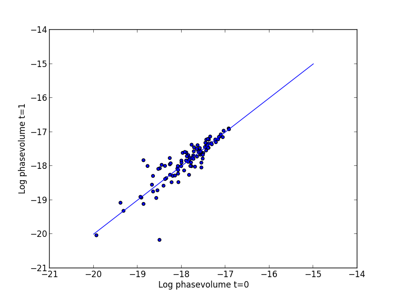
The volume at t=0 and t=1 is statistically 1. This prove the phase space volume does not change along a trajectory.