G-factor and its matrix

Note

Below is the information now upgrading (on 110315). Unfortunately serious algorithm problem is found, and thus the development is stacked so far.

G-factor is also discussed in How to calculate g-factor for H recipe. However, the above description is one of the simplest and ideal interpretation.

Now we want to introduce the G-factor in a matrix form.

Review of g-factor

It must be known for people for data analysis that the existing sensor is not perfect. One important point is that the observed count rate of the corresponding energy step is indeed an integral of the flux over the energy range.

The most generalized form to calculate the count rate for the specific energy step, i, and the direction channel, s, is

(1)\[ C_{s,i} = \int\!\!\int\!\!\int\!\!\int J(E, S, \Omega, t)\cdot k_{s,i}(E, S, \Omega) ~ dE~dS~d{\Omega}~dt\]

Here, E is the energy, S is the area of the detector, \(\Omega\) is the solid angle, t is the time. J is the differential flux, which is the function of these parameters. \(k_{s,i}\) is the response function (note that this is also in the differential form).

For simplicity, one can concentrate on the direction channel, s. This means that the s in the above equation (1) can be emitted for now.

\[C_i = \int\!\!\int\!\!\int\!\!\int J(E, S, \Omega, t)\cdot k_i(E, S, \Omega) ~ dE~dS~d{\Omega}~dt\]

Usually, g-factor is calculated by assuming that the differential flux J is constant over the range of integral and the responce, k is constant over the range of the direction (\(\Omega\)) and the area (S), meaning that:

\begin{eqnarray*} C_i &=& J(E_i) \cdot \int K_i(E) dE \cdot ~{\Delta}S~{\Delta}{\Omega}~{\Delta}t \\ &=& J(E_i) \cdot g_{e,i} \cdot {\Delta}t \\ &=& J(E_i) \cdot G_{i} \cdot E \cdot {\Delta}t \end{eqnarray*}

Here, g-factor(s) is defined like

\[ \begin{align}\begin{aligned}g_{e,i} = \int\!\!\int\!\!\int k_i(E, S, \Omega) dE~dS~d\Omega \sim \int K_i(E) dE ~{\Delta}S~{\Delta}{\Omega}\\G_i = \frac{g_{e,i}}{E_i}\end{aligned}\end{align} \]

The reasons of the introducing Gi are 1) that the center of the energy, Ei, is more handy to be used compared to the extent of the energy range, and 2) that this value becomes (rather) constant for electrostatic analyzer. However in the following, we mainly use ge,i.

Note

For CENA, the latter is not true, because the response is strongly depend on the energy. However, people is used to use the \(G_i\) value as a “g-factor”, so we follow this custom.

Finite extent of the observation space

Now we know the simplest way of the conversion between flux and count.

(2)\[ \frac{C_i}{\Delta t} = J(E_i) \cdot g_{e,i}\]

(3)\[ g_{e,i} = \int K_i(E) dE ~{\Delta}S~{\Delta}{\Omega}\]

Equation (3) is given by the sensor properties only. The values are given by (or can be derived from /TBD/) the calibration report. Equation (2) uses the g-factor, and the observed flux (left hand side) can be converted to the flux.

However, remember that the energy extent is finite. If we accept this fact, the formulations above should be written like:

(4)\[ \frac{C_i}{\Delta t} = \int J(E) \hat{g}_i(E) dE\]

Here, the new g-factor (say, differential g-factor) is being introduced.

\[\hat{g}_i(E) = \int\!\!\int k_i(E, S, \Omega) ~dS~d\Omega\]

It should be stated that the general form of the \(\hat{g}_i(E)\) should be known only by ground calibration, and sometimes it is not known. For CENA case, the most reliable source would be, for time being, Kazama-san’s simulation ([Kazama-2006]).

Warning

Now the calibration report has been issued.

If you look at the equation (4), you may notice that the count rate obesrved at energy step i is integral of the all energy range. Yes, you are right. This is a convolution form. Now you can assume the integral to be a summation.

(5)\[ \frac{C_i}{\Delta t} = \sum_{j} J(E_j) \hat{g}_i(E_j) \Delta E_j\]

If you are used to write in a matrix form, one can write

\begin{eqnarray*} \frac{1}{\Delta t} \left[ \begin{array}{c} C_0 \\ C_1 \\ \vdots \\ C_{15} \\ \end{array} \right] = \left[ \begin{array}{cccc} \hat{g}_0(E_0)\Delta E_0 & \hat{g}_0(E_1)\Delta E_1 & \cdots & \hat{g}_0(E_{15})\Delta E_{15} \\ \hat{g}_1(E_0)\Delta E_0 & \hat{g}_1(E_1)\Delta E_1 & \cdots & \hat{g}_{15}(E_{15})\Delta E_{15} \\ \vdots & \vdots & \ddots & \vdots \\ \hat{g}_{15}(E_0)\Delta E_0 & \hat{g}_{15}(E_1)\Delta E_1 & \cdots & \hat{g}_{15}(E_{15})\Delta E_{15} \\ \end{array} \right] \cdot \left[ \begin{array}{c} J_0 \\ J_1 \\ \vdots \\ J_{15} \\ \end{array} \right] \end{eqnarray*}

Here I used a syntax Jj as J(Ej). The matrix, G, can be called (internally) energy g-factor matrix. The unit is [cm^2 sr eV].

CENA energy response shape

The most reliable source of the energy response shape is in [Kazama-2006]. The shapes are in Figures 16-18.

The Figures in Kazama 2006 shows the energy response is triangle shape. Even though the peak looks rather flat and there is high energy tail, but the whole shape could be reproduced by a triangle.

However, the parameters are not exactly known. From exercises saved in scripts/cena_energy_responce_kazama.py, the parameters are likely

Beam Energy	Limit0	Peak	Limit1
25 eV	12.5 (0.5)	25 (1.0)	62.5 (2.5)
750 eV	325 (0.5)	750 (1.0)	1650 (2.2)
3300 eV	1650 (0.5)	3000 (0.91)	4950 (1.5)

Considering this result, one can assume the lower limit and peak is constant over the energy. \(L0=0.5\) and \(P=1.0\) where L0 and P is the lower limit and the peak.

Rather, Limit1 (=:math:L1)is energy dependent, and this determines the energy resolution. Only three values are available, but the \(\log(L1)\) is proportinal to the beam energy, E. \(\log(L1)=aE+b\) and considering the above parameter in the able table, a=-0.00015597 and b=0.9202 from 25 and 3300 eV. \(L1 = \exp(aE+b) = \exp(aE) + \exp(b) = 2.510\exp(-0.00015597E)\). Substituting 750 eV, L1=2.23 is obtained and this is not a bad value.

Conclusion. The energy responce in Kazama 2006 may be approximated by the triangle shaped function with the parameters as

\[\begin{split}L_0=0.5\times E_b \\\end{split}\]

\[\begin{split}L_1=2.510 \exp(-1.5597\times 10^{-4} E_b) \\\end{split}\]

\[P=E_b\]

where Eb is the beam energy, L_0 and L_1 is the bottom two points of the triangle, and P is the peak of the triangle.

CENA g-factor matrix, absolute value

Indeed, it is not yet completed. I intented to skip the issue on the absolute value. This is for equation (3).

The approach is not very clear, particularly when very small gound calibration is available, but we will anyway try it.

What is the integral g-factor (classical one, \(g_{e,i}\))? This is the conversion factor between the flux of the specific energy and the obtained count rate at the specific sensor channel. Assuming constant flux over the full energy range, the integral between the flux and the response is the g-factor.

Extending this idea, the integral over the full energy range can be used as a normalization factor of the g-factor for the matrix.

\[g_{e,i} = \sum \hat{g_i}(E_j)\Delta E_j\]

Indeed, there is another option to integrate along the direction of i, however, it may be less physical, while the results does not significantly changed.

Conversion

Now, more accurate flux considering the finite range of the energy step response can be retrieved from the count rate. Just take the inversion for the matrix.

\[\mathbf{J} = [\hat{g}_i(E_j)\Delta E_j]^{-1} \frac{\mathbf{C}}{\Delta t}\]

Note that the \(\Delta E_j\) should be taken as a range between the boundaries to the neighboring energy steps of the energy step of interst. This is obvious if you go to the equation (5).

A sample

See cena_count_rate_energy_band script.

Todo

Write down description.

A sample (old)

Warning

Below to e checked again. 2012-01-13

As a sample, we try to implement the matrix. Let’s try to calculate the energy g-factor matrix G for CH-3.

The pyana.cena.gfactor module has several ways of getting the g-factor.

>>> from pyana.cena import gfactor
>>> gf = gfactor.GFactorH_Component()
>>> g_ch3 = gf.geometricFactor()[:, 3]
>>> print g_ch3
[  2.33101872e-07   2.41815961e-07   2.54887094e-07   2.72315271e-07
   3.00636059e-07   3.42027980e-07   4.05205123e-07   4.98881576e-07
   6.38306995e-07   8.49623645e-07   1.16550936e-06   1.63824867e-06
   2.34844690e-06   3.41374424e-06   5.01060098e-06   7.40697537e-06]

Here g_ch3 is the (complete) g-factor (unit of cm2 sr eV/eV), Gi for channel 3. By multiplying Ei, you can get the energy g-factor, ge,i (unit of cm2 sr eV).

>>> from pyana.cena import energy
>>> energy_in_eV = energy.getEnergyE16()
>>> print energy_in_eV
[    7.    11.    17.    25.    38.    57.    86.   129.   193.   290.
   435.   652.   978.  1467.  2200.  3300.]

>>> ge_i = g_ch3 * energy_in_eV
>>> print ge_i
[  1.63171310e-06   2.65997557e-06   4.33308059e-06   6.80788177e-06
   1.14241702e-05   1.94955949e-05   3.48476406e-05   6.43557233e-05
   1.23193250e-04   2.46390857e-04   5.06996571e-04   1.06813813e-03
   2.29678106e-03   5.00796279e-03   1.10233222e-02   2.44430187e-02]

To obtain the g-factor matrix, the response shape of the energy step should be needed. Unfortunately we have no reliable data. So for exercise, we assume a triangular shape of the distribution. The center of the distribution is the center of the energy channel, Ei, and the range of half maximum to be (0.6 … 1.6) Ei according to the calibration report. This means that the response will be zero below 0.2 Ei and above 2.2 Ei. This is indeed also implemented in pyana.cena.energy.response_simple_triangle().

Note

I have also tried to use a Maxwellian, but it was failed, because of long tails in the low energy part. The long tails strongly affect the count rate.

Also I should mention that the “very narrow” Maxwellian, which can be used as a proxy to the scalar gfactor approximation is tried, and confirmed that the script is working.

The shape of the energy response, for energy step 8 for example, can be instanced as

>>> import math
>>> ei = energy_in_eV[8]
>>> def shape_triangle(x):
...    if x < 0.2 * ei:
...        return 0
...    elif x < ei:
...        return ((x - ei) / (0.8) + ei) / ei
...    elif x < 2.2 * ei:
...        return ( ei - (x - ei) / (1.2)) / ei
...    else:
...        return 0
>>> shape_energy_response = shape_triangle

In this case, relative g-factor matrix component, \(\hat{g}_8(E_j)|_\mathrm{rel}\), for energy step 8 can be simply derived by substitution.

>>> import numpy as np
>>> g8_j = np.array([shape_energy_response(ej) for ej in energy_in_eV])
>>> print g8_j
[ 0.          0.          0.          0.          0.          0.11917098
  0.30699482  0.58549223  1.          0.58117444  0.          0.          0.
  0.          0.          0.        ]

This is a relative value, so normalization is needed. Let’s use gfactor_norm_sum.

Warning

Indeed, this is the wrong normalization. This is along the direction of i. See also gfactor_absolute.

Now the module pyana.cena.cena_flux support the conversion from the flux to the count rate. See pyana.cena.cena_flux.Flux2Count_Matrix for details.

>>> delta_e = energy.getDeltaE16()
>>> print delta_e
[    3.05948832     4.89982994     6.9407338     10.20654189    15.7182351
    23.47397914    35.31377468    52.45977329    78.79196403   118.59621644
   177.38384309   265.97380036   399.26682807   598.69610637   897.94212647
  1347.21935853]

>>> g8_j_sum = (g8_j * delta_e).sum()
>>> g8_j = g8_j / g8_j_sum * ge_i[8]
>>> print g8_j
[  0.00000000e+00   0.00000000e+00   0.00000000e+00   0.00000000e+00
   0.00000000e+00   7.64358298e-08   1.96905344e-07   3.75532555e-07
   6.41396311e-07   3.72763141e-07   0.00000000e+00   0.00000000e+00
   0.00000000e+00   0.00000000e+00   0.00000000e+00   0.00000000e+00]

Note

In practice, CENA has not used step-0. In addition, I now realized that the CENA observation is under-determination for this approach, because only 8 energy steps are used at a time. One should think more carefully on this issue.

Same exercise can be done for different channels also.

>>> Mij = np.zeros([16, 16])
>>> for i in range(16):
...     ei = energy_in_eV[i]
...     def shape_triangle(x):
...         if x < 0.2 * ei:
...             return 0
...         elif x < ei:
...             return ((x - ei) / (0.8) + ei) / ei
...         elif x < 2.2 * ei:
...             return ( ei - (x - ei) / (1.2)) / ei
...         else:
...             return 0
...     gi_j = np.array([shape_energy_response(ej) for ej in energy_in_eV])
...     gi_j_sum = (gi_j * delta_e).sum()   # Again this is not true, normalize along another axis.
...                                         # But not significant.
...     gi_j = gi_j / gi_j_sum * ge_i[i]
...     Mij[i, :] = gi_j * delta_e
>>> print Mij
[[  8.87335353e-07   7.44377750e-07   0.00000000e+00   0.00000000e+00
    0.00000000e+00   0.00000000e+00   0.00000000e+00   0.00000000e+00
    0.00000000e+00   0.00000000e+00   0.00000000e+00   0.00000000e+00
    0.00000000e+00   0.00000000e+00   0.00000000e+00   0.00000000e+00]
        .
        .
        .
 [  0.00000000e+00   0.00000000e+00   0.00000000e+00   0.00000000e+00
    0.00000000e+00   0.00000000e+00   0.00000000e+00   0.00000000e+00
    0.00000000e+00   0.00000000e+00   0.00000000e+00   0.00000000e+00
    5.59220585e-04   2.12800561e-03   6.09062509e-03   1.56651674e-02]]

Inversion makes the g-factor matrix to the conversion matrix.

>>> Minv = np.linalg.inv(Mij)
[[  1.63065658e+06  -1.45461860e+06   1.30738522e+06  -1.18101681e+06
    9.67547015e+05  -7.85497261e+05   6.09771118e+05  -4.65234477e+05
    3.39728688e+05  -2.36699201e+05   1.60335447e+05  -1.03567397e+05
    6.39515005e+04  -4.00023449e+04   2.41127139e+04  -6.09646945e+03]
        .
        .
        .
 [ -4.11554889e-01   1.97672964e+00  -6.25336610e+00   1.00121713e+01
   -1.05242569e+01   1.64780936e+01  -3.46929669e+01   4.40221268e+01
   -2.99596248e+01   3.79374273e+01  -8.83817414e+01   9.58628120e+01
   -3.20404428e+01   3.77665368e+01  -1.52993234e+02   1.02517505e+02]]

It looks a little bit odd, as there is meaningful minus values. However, they are theoretically ok, probably, because you need minus values to make the non-diagonal component to be 0 when you multiply Mij and Minv.

>>> print Mij.dot(Minv)
[[  1.00000000e+00   0.00000000e+00   0.00000000e+00   0.00000000e+00
    0.00000000e+00   0.00000000e+00   0.00000000e+00  -5.55111512e-17
    0.00000000e+00   0.00000000e+00   0.00000000e+00  -1.38777878e-17
    0.00000000e+00   0.00000000e+00   0.00000000e+00   0.00000000e+00]
        .
        .
        .
 [ -8.67361738e-19   1.04083409e-17   0.00000000e+00  -2.77555756e-17
   -2.77555756e-17  -5.55111512e-17   0.00000000e+00   2.22044605e-16
    5.55111512e-17  -1.11022302e-16   0.00000000e+00   0.00000000e+00
    1.11022302e-16  -2.22044605e-16   0.00000000e+00   1.00000000e+00]]

Count rate test

For the fisrt test, we assume J(E), calculate expected count rate, C_i, calculate to Jcal(E) from the expected counts, and compare between J(E) and Jcal(E).

One can assume J(E) in any form, but for simplicity, we take a typical reflection energy spectra as an example (Futaana et al., in Preparation).

A typical flux follows a bipower low.

>>> import pyana.util.bipower as bipower
>>> Jtheory = bipower.mkfunc(1.6e4, -0.15, 1.4e12, -3.25)
>>> J = np.array([Jtheory(e) for e in energy_in_eV])
>>> print J
[  1.19496525e+04   1.11663460e+04   1.04605048e+04   9.87254180e+03
   9.27155210e+03   8.72446399e+03   8.20248066e+03   7.71847543e+03
   7.26584931e+03   6.83534254e+03   3.72424249e+03   9.99593330e+02
   2.67625048e+02   7.16523050e+01   1.91979264e+01   5.13993623e+00]
>>> Cexp = Mij.dot(J) * 0.375
>>> print Cexp
[ 0.00709325  0.01100683  0.01694778  0.02516675  0.03967585  0.06370262
  0.10708022  0.18609926  0.33529443  0.54110853  0.66500625  0.63692408
  0.51993462  0.35572431  0.20977722  0.18734373]

Note that the typical backscattering flux is not too strong. So I would make “offset” of 100 times for it.

>>> Cexp = Cexp * 100

I would like to also add a random noise.

>>> np.random.seed(10000)   # To keep track.
>>> Cnoise = np.random.randn(16) * 3
>>> print Cnoise
[-3.81327192  0.52841122 -0.88864913  0.98078645 -2.92025825  0.68304301
 -2.45798413  0.32166766  2.9258329   0.24592164 -1.42986759 -4.47651462
 -1.21039484  2.0843348   0.6364584   0.27296952]
>>> Cexp = np.round(Cexp + Cnoise)
[ -3.   2.   1.   3.   1.   7.   8.  19.  36.  54.  65.  59.  51.  38.  22.
  19.]
>>> Cexp[0] = 0   # To avoid negative count rate.

Ok. Lets invert count rate to the differential flux.

>>> Jrev = Minv.dot(Cexp) / 0.375 /100   # 100 is for normalizing to the original scale.
>>> print Jrev
[ -3.36352116e+05   2.93476160e+05  -1.76727336e+05   1.28654349e+05
  -6.86228519e+04   4.63062088e+04  -7.57855498e+03   1.10738087e+04
   8.30058529e+03   6.60438508e+03   3.62645817e+03   6.97963180e+02
   3.23502678e+02   1.34320034e+02   9.51204911e+00  -1.14973562e+00]
>>> print Jrev / J   # This is a "reproductivity".  1 is reproducted.
[-28.14743907  26.28220197 -16.89472342  13.0315325   -7.40144165
   5.30762794  -0.92393451   1.43471451   1.14241088   0.96621128
   0.97374384   0.69824714   1.20879073   1.8746087    0.49547274
  -0.22368675]

Well. This is not a big difference for some good part. But obviously, negative values are annoying. Ok, let’s try nnls (non-negative least square).

>>> from scipy.optimize import nnls
>>> Jrevnnls = nnls(Mij, Cexp)[0] /0.375 / 100  # Mij, not Minv!
>>> print Jrevnnls
[  0.00000000e+00   0.00000000e+00   2.40391575e+04   7.02222383e+03
   0.00000000e+00   9.32543928e+03   9.46398389e+03   3.50983051e+03
   1.15759287e+04   5.29954443e+03   4.07747456e+03   5.49125153e+02
   3.79817568e+02   1.18345941e+02   8.81066348e+00   0.00000000e+00]
>>> print Jrevnnls / J
[ 0.          0.          2.2980877   0.71128834  0.          1.06888392
  1.15379533  0.45473106  1.59319692  0.77531512  1.09484669  0.54934856
  1.41921532  1.6516697   0.45893829  0.        ]

At least it is better.

Results on plot

The result of the above samples is shown below.

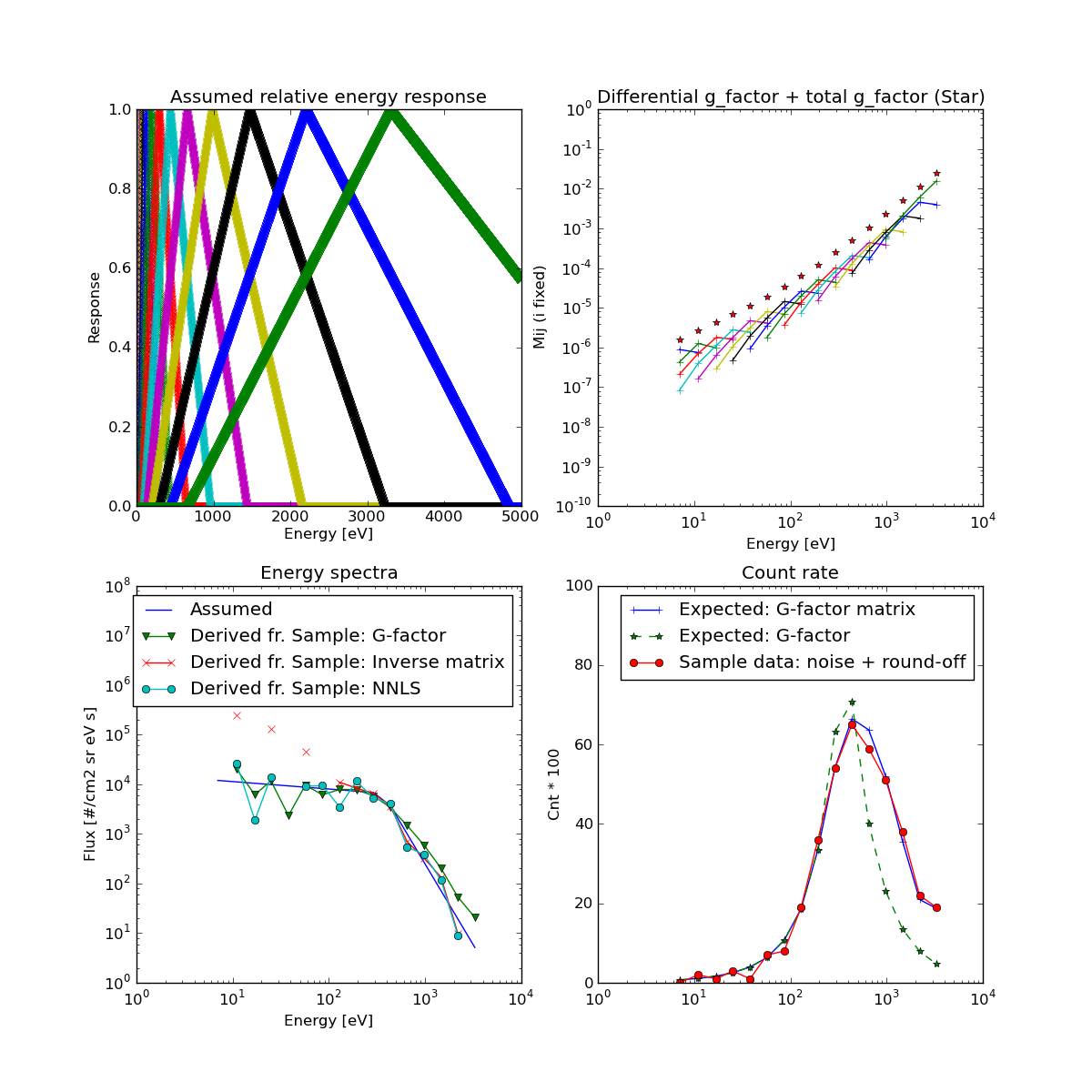
Top left shows the shape of the energy response for 16 channels. Top right shows the differential g-factor, \(\hat{g}_i(E)\). Stars are the \(g_{e,i}\). Note that they have different dimensions.

Low panels are the energy spectra and count rate. Blue in the low left panel is the assumed bi-power H-ENA spectra. They are converted to the count rate by using a energy responce (blue in low right panel). Also for comparison, we show the energy responce without considering energy channel overlap (green). Red line in the right panel shows the test data derived from the expected count rate. I assumed a small white noise and round off.

Three lines in the left panel are the derivation. Usual g-factor approach is the green line. Good reproduction in lower energy range, but not for high energy range. Using inverse g-factor matrix is the red line and symbols. Indeed, we could see fluctuation between positive and negative in the low energy part. Only positive values are shown in the log-plot. High energy part is very good. The light-blue line is using NNLS (non-negative least square) method. This reproduce the results surprisingly good.

Download the python script file (not yet clean up) from here.

Todo

Implement the module, especially considering the energy step 0 is ignored.

References

Kazama-2006(1,2)

25. Kazama. Simulation report of the ENA instrument. In IRF Scientific Report, volume 289. Swedish Institute of Space Physics, 2006.