How to calculate g-factor for H

Introduction

G-factor is important in calculating the differential flux from count rate. Details are written in the calibration report.

Theory

Theory is written in the calibration report. In the calibration report, several definition of the g-factor is defined. Usually, the g-factor is \(G_{n,i}^m\) (or \(G_{n,i}^H\)). This g-factor depends on both energy (i) and sector (n). Using 3.15, the g-factor can be used to convert between the count rate and the differential flux.

The g-factor can be separated into two part. Energy-dependent G-factor and sector-dependent part. The energy dependent g-factor is defined in 3.19.

\[G_{n,i}^{H} = \sigma{\cdot}A{\cdot}e_{i,H}{\cdot}\Bigl(\frac{\Delta E_i}{E_i}\Bigr) {\cdot}[s_n{\cdot}\Delta\Omega_n] = G_i^H {\cdot} [s_n{\cdot}\Delta\Omega_n]\]

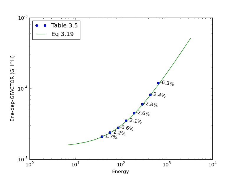
Energy dependent g-factor

Energy dependent g-factor, \(G_{i}^{H}\), can be derived by aggregating all the parameters that affect to it.

pyana.cena.gfactor module contains two derived classes: pyana.cena.gfactor.GFactorH_Table and pyana.cena.gfactor.GFactorH_Component. The difference is the way of calculation. GFactorH_Table trust Table 3.5 in the calibration report, while GFactorH_Component starts from primitive parameters.

The method energyDependentGfactor returns the energy dependent g-factor as 16-element numpy.ma.MaskedArray.

In the scripts folder, an example program is placed (cena_ene_gfactor.py).

import matplotlib
matplotlib.use('Agg')
from pylab import *

from irfpy.cena import energy
from irfpy.cena import gfactor

if __name__ == '__main__':

    # Obtain the energy in electron volts, as np.array with dimension of [16]
    energy_in_eV = energy.getEnergyE16()

    # Table-based energy dependent g-factor.
    gf0 = gfactor.GFactorH_Table()
    gf0.energyDependentGfactor()
    g0 = gf0.energyDependentGfactor()

    # Component-aggregated energy dependent g-factor.
    gf1 = gfactor.GFactorH_Component()
    gf1.energyDependentGfactor()
    g1 = gf1.energyDependentGfactor()

    diff_percent = 100 * (g1 - g0) / g0
    print(diff_percent)

    # Plot to show.
    fig = figure()
    ax = fig.add_subplot(111)
    p0 = ax.plot(energy_in_eV, g0, 'o', label='Table 3.5')
    p1 = ax.plot(energy_in_eV, g1, label='Eq 3.19')

    for i in range(len(diff_percent)):
        if not ma.is_masked(diff_percent[i]):
            ax.text(energy_in_eV[i], g0[i], ' %.1f%%' % diff_percent[i],
                                verticalalignment='center', rotation=-10)

    ax.set_xscale('log')
    ax.set_yscale('log')
    ax.set_xlabel('Energy')
    ax.set_ylabel('Ene-dep-GFACTOR (G_i^H)')

    ax.legend(loc='upper left')

    fig.savefig('cena_ene_gfactor.png')

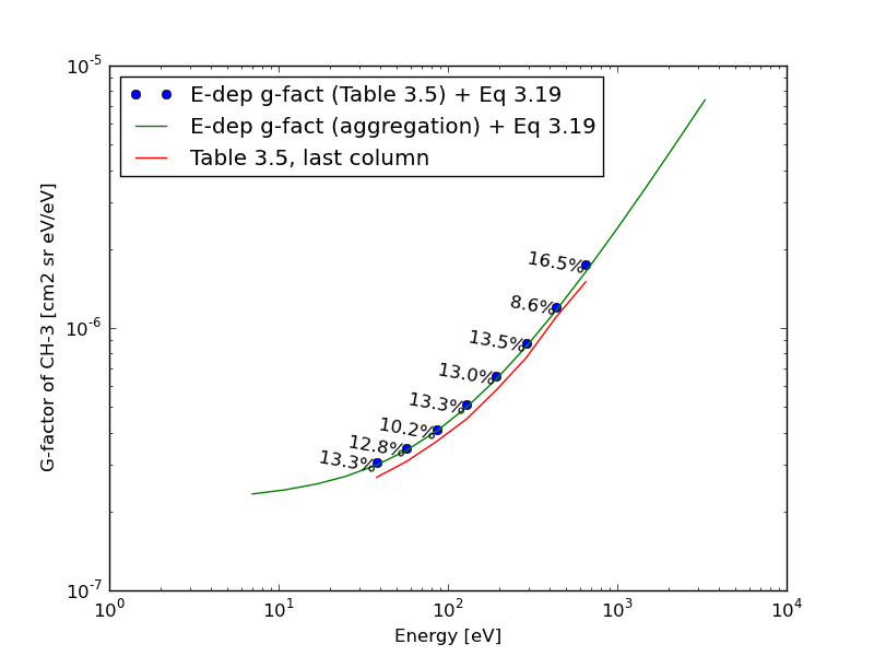
G-factor

G-factor, \(G_{n,i}^{H}\), can be calculated from the energy dependent g-factor. The geometricFactor method returns the g-factor. The returned type is numpy.ma.MaskedArray with element of [7] x [16].

There are a little confusion in the current version (issue 1 revision 1) in the calibration report. There are three calculatable g-factor values.

1. Using the energy dependent g-factor first, and derive g-factor (pyana.cena.gfactor.GFactorH_Table)

2. Using the energy dependent g-factor first, and derive g-factor (pyana.cena.gfactor.GFactorH_Component)

3. Values listed in Table, only for CH-3. (Not implemented as module)

The methods 1 and 2 has little difference, while they returns ~10% larger than the g-factor (3) listed in the last column in Table 3.15 (version v1.3+feature/cena_gfactor). This is to be investigated.

import matplotlib
matplotlib.use('Agg')

from pylab import *
from irfpy.cena import energy
from irfpy.cena import gfactor

if __name__ == '__main__':
    energy_in_eV = energy.getEnergyE16()

    # Calculate the g-factor based on the E-dep g-factor from
    # Table 3.5 the eq. 3.19
    gf0 = gfactor.GFactorH_Table()
    g0 = gf0.geometricFactor()
    g0_ch3 = g0[:,3]

    # Calculate the g-factor based on the E-dep g-factor by
    # aggregation of parameters and the eq. 3.19
    gf1 = gfactor.GFactorH_Component()
    g1 = gf1.geometricFactor()
    g1_ch3 = g1[:,3]

    # G-factor of the CH-3 listed in Table 3.5
    g2 = np.array([-10, -10, -10, -10, 2.7, 3.1, 3.7, 4.5,
                5.8, 7.7, 11, 15, -10, -10, -10, -10]) * 1e-7
    g2_ch3 = ma.masked_less(g2, 0)
    g2_ch3

    # Calculate the difference between g0 and g2.

    diff = 100 * (g0_ch3 - g2_ch3) / g2_ch3

    figure()

    plot(energy_in_eV, g0_ch3, 'o', label='E-dep g-fact (Table 3.5) + Eq 3.19')
    plot(energy_in_eV, g1_ch3, label='E-dep g-fact (aggregation) + Eq 3.19')
    plot(energy_in_eV, g2_ch3, label='Table 3.5, last column')

    for i in range(4, 12):
        print(i, g0_ch3[i], diff[i])
        text(energy_in_eV[i], g0_ch3[i], '%.1f%% ' %
                diff[i], horizontalalignment='right', rotation=-10)

    yscale('log')
    xscale('log')
    xlabel('Energy [eV]')
    ylabel('G-factor of CH-3 [cm2 sr eV/eV]')
    legend(loc='upper left')

    savefig('cena_gfactor_ch3.png')

Date

2011.01.06

See also

G-factor and its matrix section for advanced g-factor analysis.