How to fit by bi-power law

Simple bi-power fitting is shown.

First of all, one should make the answer function. The parameters (answer) here is k0=10, k1=50, r0=-0.8, and r1=-1.2.

This function can be made by irfpy.util.bipower.mkfunc() function.

>>> import irfpy.util.bipower as bipower
>>> ans_func = bipower.mkfunc(10, -0.8, 50, -1.2)

Then prepare the data point. x_array should be positive, but no need of equally separated. Thus you just prepare like

>>> import numpy as np
>>> x_array = np.array([0.1, 0.2, 0.5, 0.8, 1, 1.5, 3, 8,
... 10, 15, 20, 28, 40, 60, 100, 180, 250, 280, 300, 380, 500, 1000])

In this case, exactly corresponding y_array is like

>>> y_array = np.array([ans_func(x) for x in x_array])

But this is not a fun, because the observation have normally error. Here I want to consider relative error.

>>> import random
>>> random.seed(0)   # To use the same seed for every time.
>>> y_array_we = y_array.copy()
>>> for i in range(len(y_array_we)):
...    y_array_we[i] = y_array[i] * (1 - (random.random() - 0.5))

This introduces maximum 50% error.

Now, we want to fit the data between x_array and y_array_we.

>>> prm, success = bipower.fitting(x_array, y_array_we)
>>> print prm
(9.0417497111341678, -0.77920963653747477, 51.206001614034321, -1.2492721916019021)
>>> print success
2

Ok. Relatively good results. Now you can instance the fitted function as

>>> fitted = bipower.mkfunc(prm[0], prm[1], prm[2], prm[3])
>>> y_array_fitted = [fitted(x) for x in x_array]

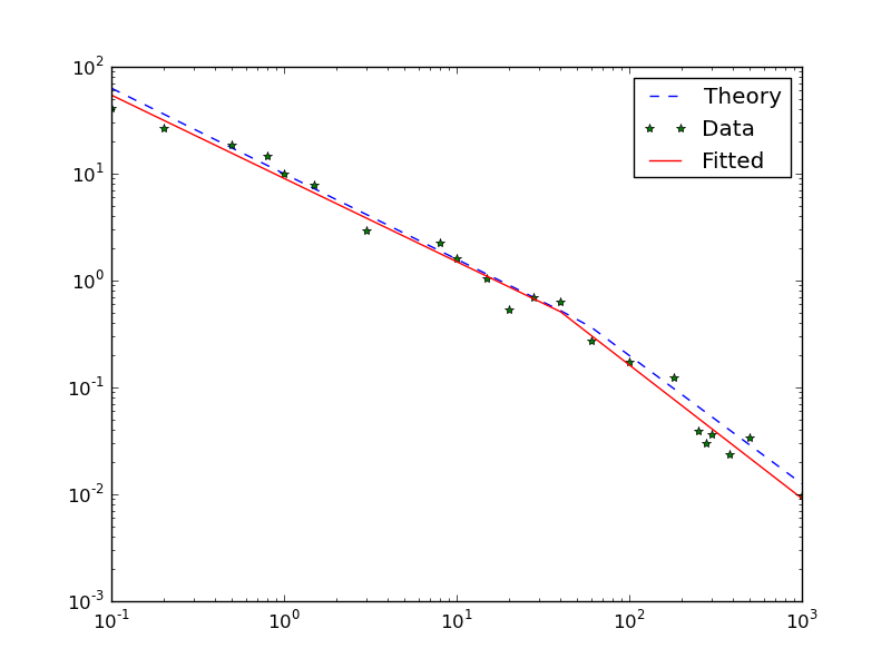
You can plot these results by matplotlib.

>>> from pylab import *
>>> plot(x_array, y_array, '--', label='Theory')
>>> plot(x_array, y_array_we, '*', label='Data')
>>> plot(x_array, y_array_fitted, '-', label='Fitted')
>>> xscale('log')
>>> yscale('log')
>>> legend()

The graph shows