snippet_cpem.plot_density_meridian

A sample file to plot the density profile.

The sample below will produce the following figure.

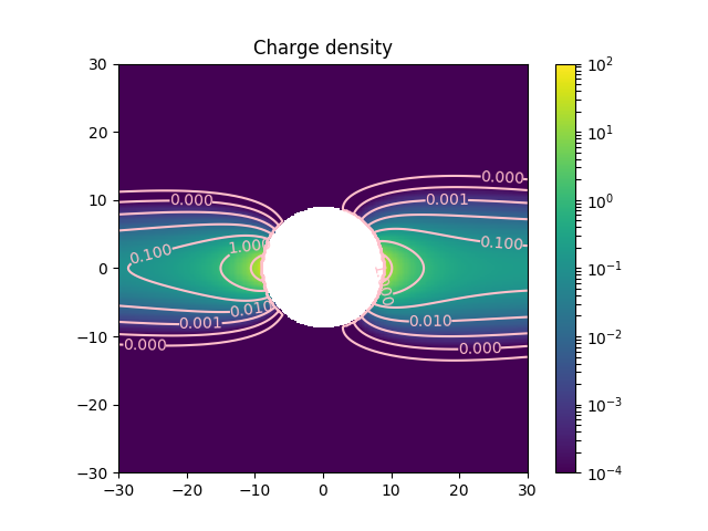
This figure shows the charge density full model of 50% percentile for MLT=0 and 12.

""" A sample file to plot the density profile.

The sample below will produce the following figure.

.. figure:: ../../../src/scripts/snippet_cpem/plot_density_meridian.png

    This figure shows the charge density full model of 50% percentile for MLT=0 and 12.
"""

import numpy as np
import matplotlib.pyplot as plt
from matplotlib.colors import LogNorm
from irfpy.cpem import cpemv2


def main():
    xp = np.linspace(-30, 30, 300)    # X grid
    yp = np.linspace(-30, 30, 299)    # Y grid

    x2p, y2p = np.meshgrid(xp, yp, indexing='ij')     # Two 1-D axes become matrix now.  Shape is (300, 299). Order x->y

    radius = np.sqrt(x2p ** 2 + y2p ** 2)     # R in each grid.
    mlat = np.degrees(np.arctan2(y2p, np.abs(x2p)))   # Magnetic latitude in degrees in each grid.
    mlt = np.where(x2p >= 0, 0, 12)     # For positive x, the MLT is 0, and negative x, the MLT is 12 hr.

    p = 0.5   # 50% percentile

    n = np.zeros_like(x2p) - 1    # The output should have the shape of (300, 299)

    # Here is the calculation
    for _ix in range(len(xp)):
        for _iy in range(len(yp)):
            _r = radius[_ix, _iy]
            if _r < 9:    # THe model is valid only for >9.
                continue
            _mlat = mlat[_ix, _iy]
            _mlt = mlt[_ix, _iy]
            n[_ix, _iy] = cpemv2.plasma_density.full_model(_r, _mlt, _mlat, p)

    plt.subplot(aspect=1, title='Charge density', ylim=[-30, 30], xlim=[-30, 30])
    pc = plt.pcolor(xp, yp, n.T, norm=LogNorm(vmin=1e-4, vmax=1e2))
    cs = plt.contour(xp, yp, n.T, np.logspace(-5, 2, 8), colors='pink', linewidth=0.5, linesytle='dashed')
    plt.clabel(cs, inline=1)

    plt.colorbar(pc)

    plt.savefig('plot_density_meridian.png')


if __name__ == '__main__':
    main()