Geometic factor

Data analysis of particle data is a fight to g-factor.

Now, irfpy.util.plasmasensor will support g-factor related issues.

Note

As of current experience, it is very difficult to generalize the discussion. This is mainly because the definition of the g-factor is highly up to the person.

Convert J to C

What I want to do here is to convert the differential flux to the count rate.

The differential flux, \(J\) [/cm^2 sr eV s] is supposed to be given in 3-D space, namely, \(J=J(E, \theta, \phi)\). When the differential flux is measured by a plasma sensor, the counts of specific bin is given as

\[C/\Delta t=\int\int\int\int J(E, \theta, \phi)\cdot k^*(E, \theta, \phi)~dE~dS~d^2\Omega\]

Therefore, the question is solved by knowing \(k^*(E, \theta, \phi)\) for each bins. The unit of this quantity (\(k^*\)) is [1] (unitless). The quantity is equivalent to efficiency, and sometimes called energy/angular response function. This information can only be obtained from ground calibration.

The g-factor is the approximation of this equation. Assume \(J\) does not depend on \(E, \theta, \phi\) over the (effective) integration range. Then, you may modify the equation above to

\[\begin{split}C/\Delta t &= J(E_0, \theta_0, \phi_0) \int\int\int\int k^*(E, \theta, \phi)~dE~dS~d^2\Omega \\ &= J K \Delta E~\Delta S~\Delta \Omega \\ &= J K G E\end{split}\]

Here, \(G=(\Delta E / E) \Delta S \Delta \Omega\) is almost constant over the energy. This is called “geometric factor (efficiency excluded)” and \(K G\) is “geometric factor (efficiency included)”.

For example, MEX/IMA case, the geometric factor (eff. incl.) is 3.5e-4 cm2 sr eV/eV.

Warning

This could be a wrong sentence. It rather makes sense to consider 3.5e-4 is only cm2 sr, without eV/eV. TBC

Sometimes the efficiency (energy/angular response) is given by the function that is normalized so as to make the maximum 1. But it is obvious that the absolute efficiency should be scaled to satisfy

\[\int\int\int\int k^*(E, \theta, \phi)~dE~dS~d^2\Omega = K G E\]

Example

Let us see an example.

Consider a plasma sensor’s bin with the g-factor (incl eff) as 3.5e-4 cm2 sr eV/eV. Suppose the energy bin is 200 eV. Let us consider \(\Delta S=\) 0.1 cm2. Finally from a calibration, we get the following response function.

\[\begin{split}\epsilon &= 1 (190 < E < 210 eV \& -5 < \theta < 5 \& -10 < \phi < 10) \\ \epsilon &= 0 (otherwise) \\\end{split}\]

What is the \(k^*\) for this sensor’s bin?

Answer

Ok, first, \(K G E= 3.5\times 10^{-4} \times 200 = 7\times 10^{-2}\) cm2 sr eV.

\[\begin{split}KGE &= \int\int\int\int k^*(E, \theta, \phi) dEdSd^2\Omega \\ &= \int\int\int\int \kappa \epsilon(E, \theta, \phi) dEdSd^2\Omega \\ \kappa &= \frac{KGE}{\int\int\int\int \epsilon(E, \theta, \phi) dEdSd^2\Omega}\end{split}\]

The integral part can be solved simply in this case. Numerical calculation might be needed for actial cases. Nevertheless, dE = 20 eV, dS = 0.2 cm2, and dOmega ~ 0.08 sr, so that the integral part is 0.32 sr cm2 ev. Thus, \(\kappa = 0.07 / 0.32 = 0.22\).

Answer: \(k^* = 0.22\) for E in 190-210 eV and \(\theta\) in -5 and 5 degrees and \(\phi\) in -10 and 10 degrees. Otherwise 0.

Also in this case, \(max(k^*) = K\) where K is the averaged efficiency.

Sample code

Let us think the sample code. See scripts.sample_130911_gfactor.

More realistic application

Here I describe more realistic application.

For the ideal efficiency response to energy/angle should be

• Flat topped (if the observation is not exactly the center, the response should be kept)

• Quick reduction (if the observation is done far from the center, the response should be 0)

• Easy to implement/calculate. Small number of paramters.

• Or, tabulated.

The last one is the request from the computational resource.

While there are no single answer, “general gaussian” form may be used, for example.

\[k^*(E, \theta, \phi) = \prod_{V=E,\theta,\phi}\exp\Bigl(-\frac{1}{2}\Bigl|\frac{V}{\sigma_V}\Bigr|^{2p_V}\Bigr)\]

The function is implemented by scipy. http://docs.scipy.org/doc/scipy-dev/reference/generated/scipy.signal.general_gaussian.html

The half-power-point is at

\[n_\mathrm{h} = \sigma(2\ln 2)^\frac{1}{2p}\]

so that the FWHM is \(2n_\mathrm{h}\). From this value, you may guess the \(\sigma\) as

\[\sigma = \frac{\mathrm{FWHM}}{2(2\ln 2)^\frac{1}{2p}}\]

IMA/MEX & VEX

Ok, let us think “IMA” sensor. Assume a bin. Mass direction is collapsed for simplicity. This is not a bad assumption if one handles solar wind. Now, the bin should have a response function, \(k^*\).

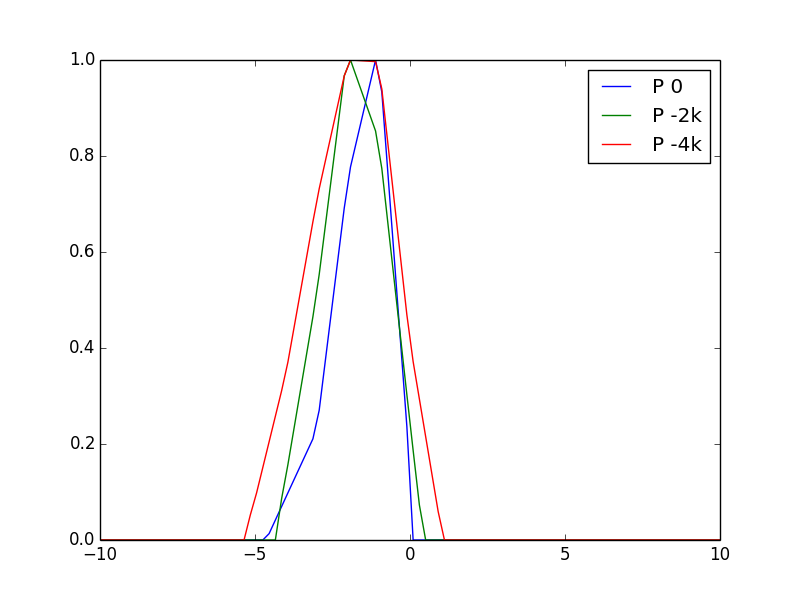
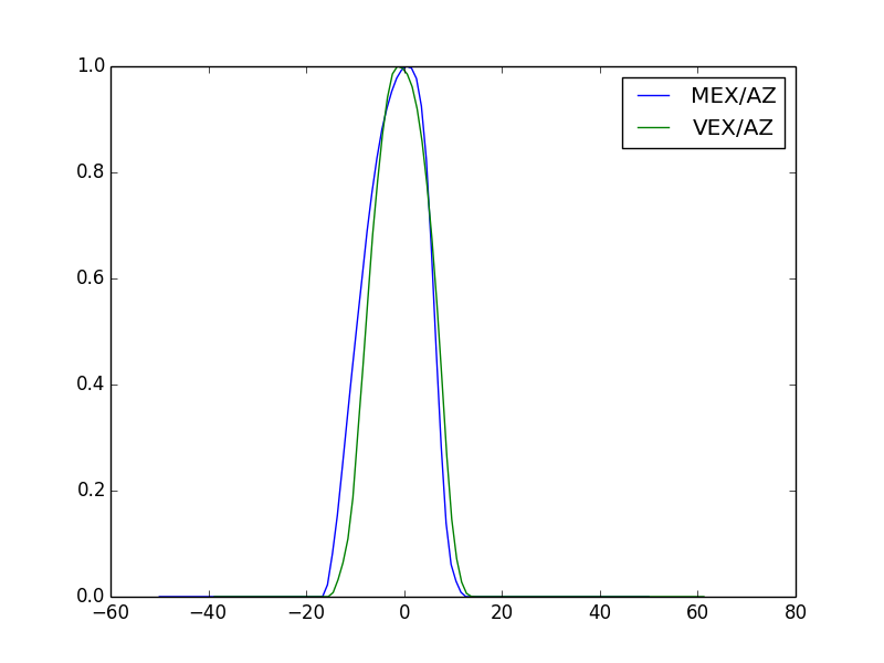
Azimuth and Polar

The azimuth angle dependence can be seen at Fig 29 in Barabash et al., 2007 for VEX. In Fig. 30 in Barabash et al., 2007, elevation and azimuth response is seen.

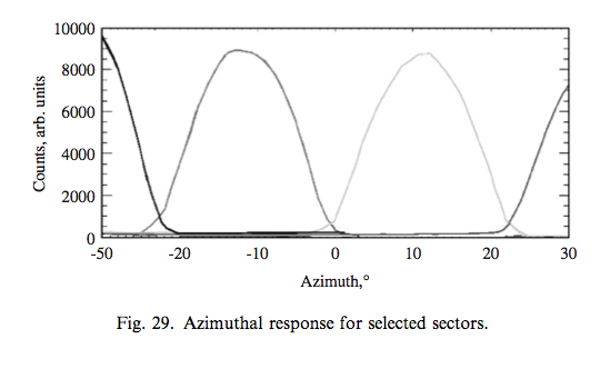
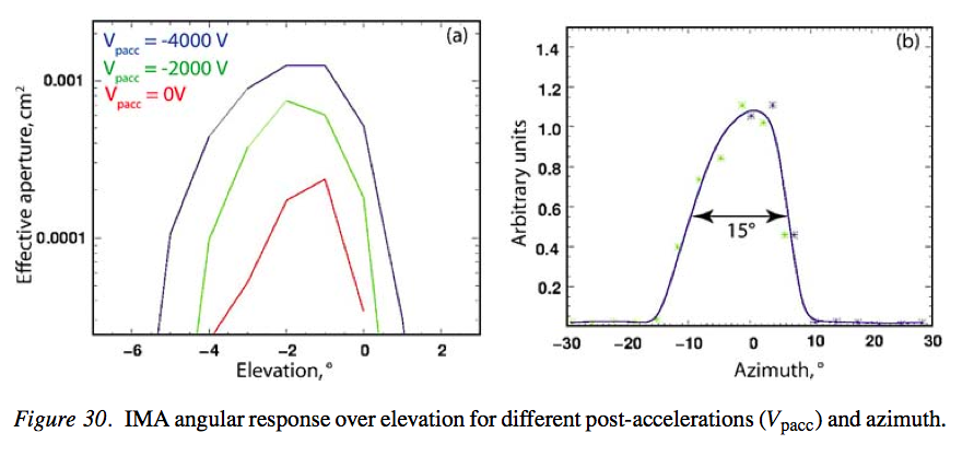
Using the g3data and linear interpolation, implementation is in irfpy.vima.efficiency0.VimaAzimResp, irfpy.mima.efficiency0.MimaAzimResp, and irfpy.mima.efficiency0.MimaElevResp.

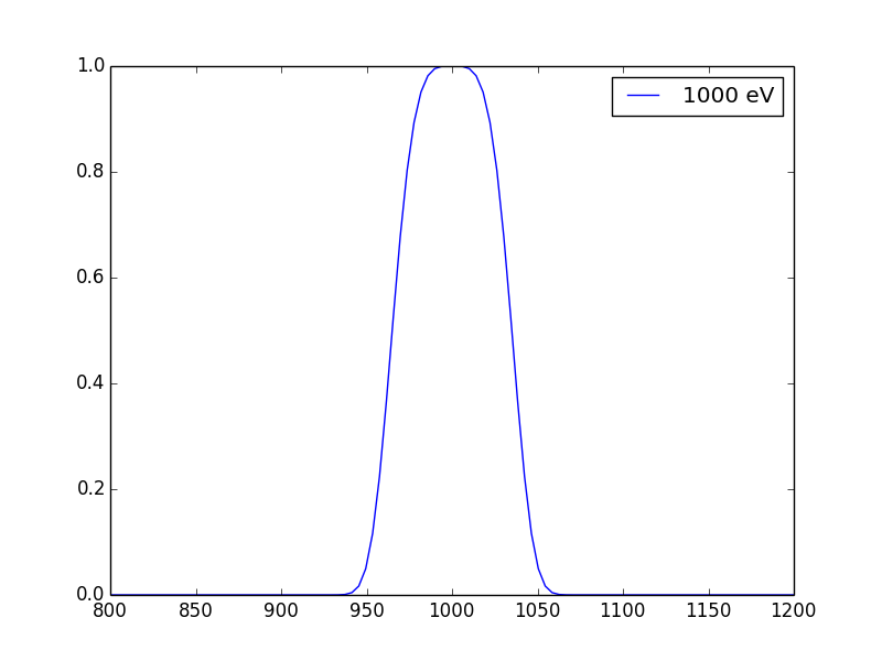
Energy

I do not have good reference on it. So that my guess work is here.

Ok, assume the center energy, \(E_0 = 1000\) [eV].

The energy resolution is to be 7%, and take this value as FWHM (\(0.07E_0\)). We here presumably put \(p_E=2\). Now, you may get the \(\sigma_E=0.0322 E_0 = 32.2\).

This is implemented in irfpy.mima.efficiency0.MimaEnerResp.